Time Series Forecasting with Long Short-Term Memory (LSTM) Networks in TensorFlow

Time series forecasting is a critical aspect of predictive analytics, finding applications in diverse domains such as finance, weather prediction, and resource planning. As the need for accurate predictions from sequential data grows, machine learning techniques like Long Short-Term Memory (LSTM) networks have become indispensable. This blog aims to provide a comprehensive guide to implementing LSTM networks for time series forecasting using the TensorFlow library.

What is Time Series Data?

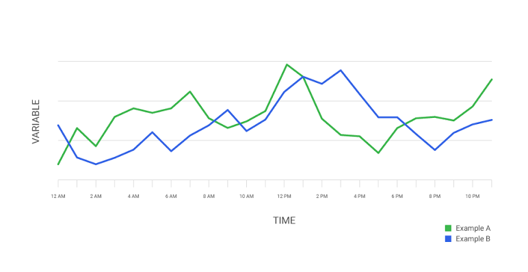
Time series data represents observations recorded over time, creating a sequence of data points. Recognizing patterns and dependencies within this temporal structure is crucial for effective forecasting. Time series data often exhibits trends, seasonality, and irregular fluctuations, making it different from traditional datasets.

Consider a scenario where you want to predict daily stock prices. Each day’s closing price depends on previous prices and external factors, illustrating the sequential nature of time series data. Recognizing these dependencies is fundamental for selecting appropriate models.

Introduction to Long Short-Term Memory (LSTM) Networks

Traditional neural networks struggle with sequential data due to their inability to retain context over long sequences. Recurrent Neural Networks (RNNs) were introduced to address this limitation but faced challenges in training long sequences due to the vanishing gradient problem. LSTM networks were designed to overcome these challenges.

Key Principles of LSTMs

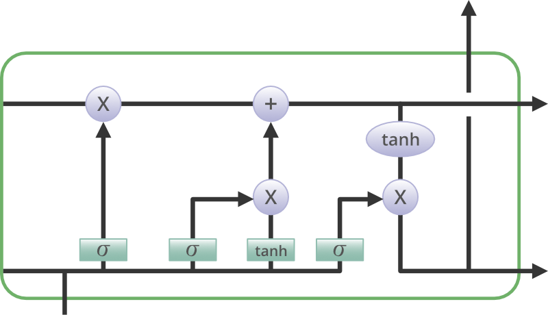
Memory Cells: LSTMs contain memory cells that can store and retrieve information over long sequences.

Gates: Forget, input, and output gates control the flow of information, allowing LSTMs to selectively remember or forget.

TensorFlow Basics

TensorFlow, an open-source machine learning library developed by Google, provides a robust platform for building and training various machine learning models. Before diving into LSTM networks, let’s cover some essential TensorFlow basics.

Installing TensorFlow

You can install TensorFlow using pip:

bash

pip install tensorflow

Building a Simple Neural Network

Let us create a basic neural network using TensorFlow’s Keras API:

python

import tensorflow as tf

from tensorflow.keras import layers, models

# Define a simple neural network

model = models.Sequential([

    layers.Dense(32, activation=’relu’, input_shape=(input_dim,)),

    layers.Dense(1)  # Output layer

])

# Compile the model

model.compile(optimizer=’adam’, loss=’mean_squared_error’)

Preparing Time Series Data for LSTM

Properly preparing time series data is crucial for the success of an LSTM model. Let’s go through the necessary steps:

Importing Libraries

python

import numpy as np

import pandas as pd

from sklearn.model_selection import train_test_split

from sklearn.preprocessing import MinMaxScaler

Loading Time Series Data

Load the time series data from a CSV file:

python

# Load time series data

data = pd.read_csv(‘time_series_data.csv’)

# Display the first few rows of the dataset

print(data.head())

Preprocessing Steps

python

Copy code

# Extracting the target variable

target_variable = data[‘target’].values

# Scaling the target variable

scaler = MinMaxScaler(feature_range=(0, 1))

scaled_target = scaler.fit_transform(target_variable.reshape(-1, 1))

# Splitting the data into training and testing sets

train_data, test_data = train_test_split(scaled_target, test_size=0.2, shuffle=False)

Creating Sequences and Labels

python

def create_sequences_and_labels(data, sequence_length):

    sequences, labels = [], []

    for i in range(len(data) – sequence_length):

        sequence = data[i:i + sequence_length]

        label = data[i + sequence_length]

        sequences.append(sequence)

        labels.append(label)

    return np.array(sequences), np.array(labels)

# Define sequence length

sequence_length = 10

# Create sequences and labels for training set

X_train, y_train = create_sequences_and_labels(train_data, sequence_length)

# Create sequences and labels for testing set

X_test, y_test = create_sequences_and_labels(test_data, sequence_length)

Implementing LSTM for Time Series Forecasting in TensorFlow

Now that the data is prepared, let’s build and train an LSTM model using TensorFlow’s Keras API.

Building the LSTM Model

python

from tensorflow.keras.models import Sequential

from tensorflow.keras.layers import LSTM, Dense

model = Sequential([

    LSTM(50, activation=’relu’, input_shape=(X_train.shape[1], 1)),

    Dense(1)

])

model.compile(optimizer=’adam’, loss=’mean_squared_error’)

Training the Model

python

model.fit(X_train, y_train, epochs=50, batch_size=32, validation_data=(X_test, y_test))

Model Evaluation

After training the model, it’s essential to evaluate its performance on the testing set.

python

# Predictions on the testing set

y_pred = model.predict(X_test)

# Inverse transform the scaled predictions

y_pred = scaler.inverse_transform(y_pred)

y_test = scaler.inverse_transform(y_test.reshape(-1, 1))

# Calculate Mean Absolute Error (MAE) and Root Mean Squared Error (RMSE)

mae = np.mean(np.abs(y_test – y_pred))

rmse = np.sqrt(np.mean((y_test – y_pred) ** 2))

print(f’Mean Absolute Error (MAE): {mae}’)

print(f’Root Mean Squared Error (RMSE): {rmse}’)

Model Interpretation and Visualization

Understanding how the LSTM model arrives at predictions is crucial. Visualizing the predictions against the actual time series data can provide insights.

Plotting Predictions

python

import matplotlib.pyplot as plt

# Plotting the actual vs. predicted values

plt.figure(figsize=(12, 6))

plt.plot(y_test, label=’Actual’, color=’blue’)

plt.plot(y_pred, label=’Predicted’, color=’red’)

plt.title(‘Time Series Forecasting with LSTM’)

plt.xlabel(‘Time’)

plt.ylabel(‘Value’)

plt.legend()

plt.show()

Hyperparameter Tuning

Fine-tuning the model’s hyperparameters can significantly impact its performance. Experiment with different configurations to achieve optimal results.

Example of Hyperparameter Tuning

python

# Example of hyperparameter tuning

model = Sequential([

    LSTM(100, activation=’relu’, input_shape=(X_train.shape[1], 1)),

    Dense(1)

])

model.compile(optimizer=’adam’, loss=’mean_squared_error’)

model.fit(X_train, y_train, epochs=100, batch_size=64, validation_data=(X_test, y_test))

Handling Longer Sequences with Bidirectional LSTMs

In scenarios where capturing information from both past and future sequences is essential, Bidirectional LSTMs can be employed.

Building a Bidirectional LSTM Model

python

from tensorflow.keras.layers import Bidirectional

# Build a Bidirectional LSTM model

model_bidirectional = Sequential([

    Bidirectional(LSTM(50, activation=’relu’), input_shape=(X_train.shape[1], 1)),

    Dense(1)

])

model_bidirectional.compile(optimizer=’adam’, loss=’mean_squared_error’)

Future Improvements and Advanced Techniques

While LSTMs provide a solid foundation for time series forecasting, exploring advanced techniques can enhance predictive capabilities.

Advanced Techniques

Attention Mechanisms: Integrate attention mechanisms to allow the model to focus on specific parts of the input sequence.

Ensemble Learning: Combine predictions from multiple models to improve overall forecasting accuracy.

Conclusion

To conclude, we have explored the intricate process of implementing Long Short-Term Memory (LSTM) networks for time series forecasting using TensorFlow. From understanding the nuances of time series data to preparing the data, building an LSTM model, and evaluating its performance, every step has been elucidated with detailed code examples. The inclusion of visualization, hyperparameter tuning, and the introduction of Bidirectional LSTMs adds depth to the discussion.

Armed with this knowledge, you are now well-equipped to tackle your own time series forecasting projects, confidently leveraging the power of LSTMs and TensorFlow. As the field of machine learning continues to evolve, the application of advanced techniques and continuous exploration of new methodologies will undoubtedly shape the future of time series forecasting.