
Machine learning has become an indispensable tool in solving complex problems across various domains. Unsupervised machine learning, in particular, plays a crucial role in discovering patterns and hidden structures within data without the need for labelled examples.
In this blog, we will explore some of the most powerful unsupervised machine learning techniques in Clustering, Dimensionality Reduction, and Anomaly Detection.
Clustering Techniques
Clustering is a fundamental unsupervised learning task that groups similar data points in a dataset. The primary goal of clustering is to divide the data into meaningful clusters, enabling us to gain insights and identify patterns within the data.
Let’s explore two popular clustering algorithms:
- K-Means Clustering
- Hierarchical Clustering.
K-Means Clustering
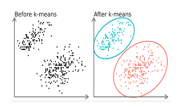
K-Means is a simple yet effective clustering algorithm. The process involves the following steps:
- Initialize K cluster centroids randomly.
- Assign each data point to the nearest centroid.
- Update the centroids by calculating the mean of data points within each cluster.
- Repeat steps 2 and 3 until convergence.
Let’s implement K-Means in Python:
Python
# Importing required libraries
import numpy as np
from sklearn.datasets import make_blobs
from sklearn.cluster import KMeans
import matplotlib.pyplot as plt
# Generate synthetic data
X, _ = make_blobs(n_samples=300, centers=3, random_state=42)
# Creating K-Means model with 3 clusters
kmeans = KMeans(n_clusters=3, random_state=42)
# Fitting the model to the data
kmeans.fit(X)
# Getting the cluster centroids and labels
centroids = kmeans.cluster_centers_
labels = kmeans.labels_
# Visualizing the clusters and centroids
plt.scatter(X[:, 0], X[:, 1], c=labels, cmap=’viridis’)
plt.scatter(centroids[:, 0], centroids[:, 1], marker=’X’, s=200, c=’red’)
plt.title(‘K-Means Clustering’)
plt.xlabel(‘Feature 1’)
plt.ylabel(‘Feature 2’)
plt.show()
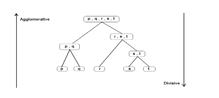
Hierarchical Clustering
Hierarchical Clustering is another powerful technique that forms a tree-like hierarchy of clusters. It can be agglomerative (bottom-up) or divisive (top-down). We will focus on the agglomerative approach, where each data point starts as an individual cluster and merges with the closest cluster until a single cluster containing all data points is formed.
Python
# Importing required libraries
import numpy as np
from sklearn.datasets import make_blobs
from scipy.cluster.hierarchy import dendrogram, linkage
import matplotlib.pyplot as plt
# Generate synthetic data
X, _ = make_blobs(n_samples=300, centers=3, random_state=42)
# Creating the linkage matrix using Ward’s method
linkage_matrix = linkage(X, method=’ward’)
# Plotting the dendrogram
plt.figure(figsize=(10, 5))
dendrogram(linkage_matrix)
plt.title(‘Hierarchical Clustering Dendrogram’)
plt.xlabel(‘Data Index’)
plt.ylabel(‘Distance’)
plt.show()
Dimensionality Reduction Techniques
High-dimensional data can be challenging to visualize and analyze. Dimensionality Reduction techniques help to overcome this problem by projecting data into a lower-dimensional space while preserving essential information. Two widely used dimensionality reduction algorithms are Principal Component Analysis (PCA) and t-Distributed Stochastic Neighbor Embedding (t-SNE).
Principal Component Analysis (PCA)
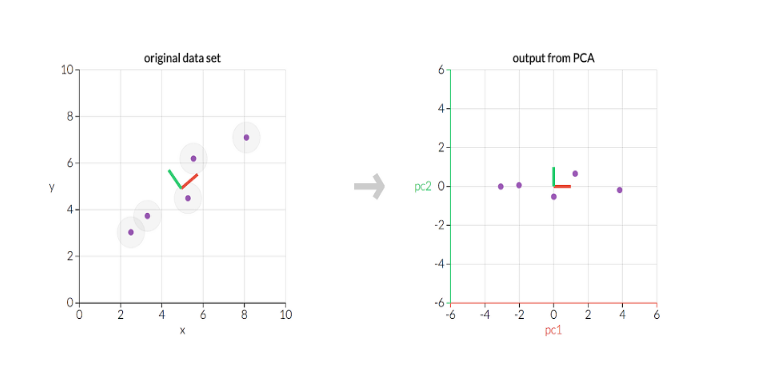
PCA is a linear dimensionality reduction technique that identifies the principal components capturing the most significant variance in the data. It transforms the original features into a new coordinate system aligned with these principal components.
Python
# Importing required libraries
import numpy as np
from sklearn.datasets import load_iris
from sklearn.decomposition import PCA
import matplotlib.pyplot as plt
# Load Iris dataset
data = load_iris()
X, y = data.data, data.target
# Applying PCA to reduce data to 2 dimensions
pca = PCA(n_components=2)
X_pca = pca.fit_transform(X)
# Visualizing the reduced data
plt.scatter(X_pca[:, 0], X_pca[:, 1], c=y, cmap=’viridis’)
plt.title(‘PCA: Iris Dataset’)
plt.xlabel(‘Principal Component 1’)
plt.ylabel(‘Principal Component 2’)
plt.show()
t-Distributed Stochastic Neighbor Embedding (t-SNE).
t-SNE is a non-linear dimensionality reduction technique particularly useful for visualization purposes.
It focuses on preserving local structures, making it excellent for revealing clusters and patterns in high-dimensional data.
Python
# Importing required libraries
import numpy as np
from sklearn.datasets import load_iris
from sklearn.manifold import TSNE
import matplotlib.pyplot as plt
# Load Iris dataset
data = load_iris()
X, y = data.data, data.target
# Applying t-SNE to reduce data to 2 dimensions
tsne = TSNE(n_components=2, random_state=42)
X_tsne = tsne.fit_transform(X)
# Visualizing the reduced data
plt.scatter(X_tsne[:, 0], X_tsne[:, 1], c=y, cmap=’viridis’)
plt.title(‘t-SNE: Iris Dataset’)
plt.xlabel(‘t-SNE Component 1’)
plt.ylabel(‘t-SNE Component 2’)
plt.show()
Anomaly Detection Techniques
Anomaly detection is the process of identifying rare and abnormal instances in a dataset, which may indicate potential fraudulent activities or system malfunctions. Two commonly used anomaly detection techniques are Isolation Forest and Autoencoders.
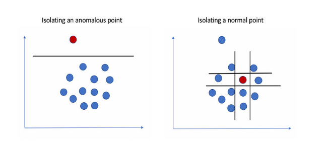
Isolation Forest
The Isolation Forest algorithm separates anomalies by randomly selecting features and partitioning data points into isolation trees. Anomalies will be isolated with a shorter average path length compared to normal data points.
Python
# Importing required libraries
import numpy as np
from sklearn.datasets import make_classification
from sklearn.ensemble import IsolationForest
import matplotlib.pyplot as plt
# Generate synthetic data
X, _ = make_classification(n_samples=300, n_features=2, n_informative=2, n_redundant=0, random_state=42)
# Creating Isolation Forest model
isolation_forest = IsolationForest(contamination=0.1, random_state=42)
# Fitting the model to the data
isolation_forest.fit(X)
# Predicting anomalies
y_pred = isolation_forest.predict(X)
# Visualizing anomalies
plt.scatter(X[:, 0], X[:, 1], c=np.where(y_pred == -1, ‘red’, ‘blue’))
plt.title(‘Isolation Forest: Anomaly Detection’)
plt.xlabel(‘Feature 1’)
plt.ylabel(‘Feature 2’)
plt.show()
Autoencoders
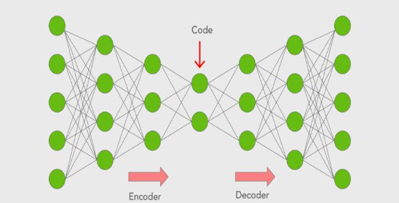
Autoencoders are neural network models used for unsupervised learning of efficient data representations. The encoder network compresses the input data into a lower-dimensional representation, while the decoder network attempts to reconstruct the original data from this compressed representation.
Anomalies will have higher reconstruction errors, making them distinguishable from normal data points.
Python
# Importing required libraries
import numpy as np
from sklearn.datasets import make_classification
from sklearn.preprocessing import MinMaxScaler
from tensorflow.keras.models import Model
from tensorflow.keras.layers import Input, Dense
import matplotlib.pyplot as plt
# Generate synthetic data
X, _ = make_classification(n_samples=300, n_features=10, n_informative=10, random_state=42)
# Normalize the data
scaler = MinMaxScaler()
X_norm = scaler.fit_transform(X)
# Define the autoencoder architecture
input_layer = Input(shape=(10,))
encoded = Dense(5, activation=’relu’)(input_layer)
decoded = Dense(10, activation=’sigmoid’)(encoded)
# Create the autoencoder model
autoencoder = Model(input_layer, decoded)
# Compile the model
autoencoder.compile(optimizer=’adam’, loss=’binary_crossentropy’)
# Train the autoencoder
autoencoder.fit(X_norm, X_norm, epochs=50, batch_size=32, validation_split=0.2)
# Reconstruct data using the trained autoencoder
X_reconstructed = autoencoder.predict(X_norm)
# Calculate reconstruction errors
reconstruction_errors = np.mean(np.square(X_norm – X_reconstructed), axis=1)
# Visualizing reconstruction errors
plt.scatter(range(len(reconstruction_errors)), reconstruction_errors, c=’blue’)
plt.axhline(y=np.percentile(reconstruction_errors, 95), color=’red’, linestyle=’dashed’, label=’Anomaly Threshold’)
plt.title(‘Autoencoders: Anomaly Detection’)
plt.xlabel(‘Data Index’)
plt.ylabel(‘Reconstruction Error’)
plt.legend()
plt.show()
Conclusion
Unsupervised machine learning techniques play a vital role in data exploration, pattern discovery, and anomaly detection. In this blog, we covered three powerful unsupervised learning techniques in Clustering, Dimensionality Reduction, and Anomaly Detection. We implemented K-Means and Hierarchical Clustering for grouping similar data points, PCA, and t-SNE for visualizing high-dimensional data, and Isolation Forest and Autoencoders for detecting anomalies. With these tools in your arsenal, you can gain deeper insights and make data-driven decisions in various applications, ranging from customer segmentation and image processing to fraud detection and system monitoring.