What is Machine Learning: Types, Learning Processes & Examples of ML

Machine Learning (ML) has become a highly influential and revolutionary technology in today’s digital era. It provides energy to various applications, such as recommendation systems in online shopping platforms and predictive models in the medical field. However, what exactly is machine learning?

ML is essentially a part of AI that allows systems to learn and enhance through experience without direct programming. ML models do not adhere to strict rules; instead, they identify patterns and base predictions or decisions on data. ML’s versatility allows it to address a wide variety of issues, including comprehending language and identifying fraudulent activities.

What is the Significance of Machine Learning?

ML’s significance comes from its capacity to manage large quantities of data and derive practical insights that humans would struggle to analyze by hand. ML frees up human effort for creative and strategic work by automating repetitive tasks.

This blog will look into:

• Different methods of machine learning techniques.
• Training ML models involves a specific set of steps.
• Instances of practical uses of machine learning in the real world.

Let us discover more about this thrilling field.

Types of Machine Learning

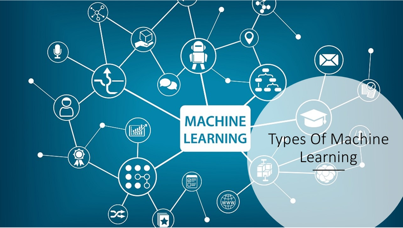
Machine Learning is broadly categorized into four types. Each type has unique characteristics suited for specific problem domains.

1. Supervised Learning

Supervised learning is the most commonly used type of ML. It works with labeled datasets, meaning the input data comes with corresponding outputs. The model learns by mapping inputs to outputs and uses this knowledge to predict outputs for unseen inputs.

Common Use Cases:

• Predicting sales figures (Regression)
• Diagnosing diseases based on symptoms (Classification)

Code Example: Linear Regression for Predicting Sales

import numpy as np
from sklearn.linear_model import LinearRegression
from sklearn.model_selection import train_test_split

# Data: Advertising spend (input) vs. Sales (output)
X = np.array([100, 200, 300, 400, 500]).reshape(-1, 1)  
y = np.array([20, 40, 60, 80, 100])

# Split data
X_train, X_test, y_train, y_test = train_test_split(X, y, test_size=0.2, random_state=42)

# Model training
model = LinearRegression()
model.fit(X_train, y_train)

# Predicting new sales

predicted_sales = model.predict([[350]])
print(f"Predicted Sales for $350 spend: {predicted_sales[0]}")

This example trains a simple model to predict sales based on advertising spend.

2. Unsupervised Learning

Unsupervised learning involves data without labels. The goal is to identify hidden patterns, group similar data points, or find correlations.

Common Use Cases:

• Market segmentation in retail.
• Identifying anomalies in network traffic.

Code Example: Clustering Customers Using K-Means

from sklearn.cluster import KMeans
import numpy as np

# Sample customer data (Age, Annual Income)
data = np.array([[22, 20], [25, 35], [40, 65], [55, 80], [23, 30]])

# Apply K-Means
kmeans = KMeans(n_clusters=2, random_state=42)
kmeans.fit(data)

# Cluster centers and labels
print("Cluster Centers:\n", kmeans.cluster_centers_)
print("Labels:", kmeans.labels_)

This code divides customers into clusters based on age and income, which businesses can use for targeted marketing.

3. 
   

   Semi-Supervised Learning

Semi-supervised learning strikes a balance between supervised and unsupervised learning. It works well when labeled data is scarce and unlabeled data is abundant.

Common Use Cases:

• Sentiment analysis for social media
• Identifying genetic disorders

Code Example: Label Propagation for Classifying Partially Labeled Data

from sklearn.semi_supervised import LabelPropagation
import numpy as np

# Partially labeled data
X = [[1, 2], [3, 4], [5, 6], [7, 8], [9, 10]]
y = [0, 1, -1, -1, -1]  # -1 means unlabeled

# Label propagation
model = LabelPropagation()
model.fit(X, y)
print("Propagated Labels:", model.transduction_)

This method propagates labels to unlabeled data based on the similarity to labeled points.

4. Reinforcement Learning

Reinforcement Learning (RL) involves training an agent to take actions in an environment to maximize cumulative rewards. Unlike other learning types, RL focuses on sequential decision-making.

Common Use Cases:

• Robotics for task automation
• AI in gaming

Code Example: Q-Learning for a Grid Navigation Problem

import numpy as np

# Define Q-table
Q = np.zeros((5, 5))  # States x Actions

# Learning parameters
alpha = 0.8  # Learning rate
gamma = 0.9  # Discount factor
rewards = np.array([[-1, -1, -1, -1, 10], [0, -1, -1, -1, 0]])  # Sample reward grid

# Update Q-values (simplified example)
for i in range(100):
    state = np.random.randint(0, 5)
    action = np.random.randint(0, 5)
    reward = rewards[0][action]
    next_state = action
    Q[state, action] = Q[state, action] + alpha * (reward + gamma * np.max(Q[next_state, :]) - Q[state, action])

print("Q-Table:\n", Q)

In this example, the Q-Table stores the optimal policy for navigating the grid.

Machine Learning Processes

1. Data Collection and Preprocessing

The performance of the model is heavily influenced by the quality of the input data. Preprocessing guarantees the dataset is tidy and can be utilized. 

Example: Handling Missing Values and Standardizing Data

import pandas as pd
from sklearn.impute import SimpleImputer
from sklearn.preprocessing import StandardScaler

data = {'Age': [25, None, 35, 40], 'Salary': [50000, 60000, None, 80000]}
df = pd.DataFrame(data)

# Impute missing values
imputer = SimpleImputer(strategy='mean')
df.iloc[:, :] = imputer.fit_transform(df)

# Standardize
scaler = StandardScaler()
df.iloc[:, :] = scaler.fit_transform(df)
print(df)

2. Feature Selection and Engineering

Feature selection and engineering are critical steps in the machine learning process, ensuring that models learn effectively from relevant data.

• Feature Selection: This process identifies the most important variables (features) in a dataset, removing redundant or irrelevant data. It reduces dimensionality, speeds up computation, and improves model accuracy. Methods include:
  • Filter Methods: Using statistical measures like correlation or variance to select features.
  • Wrapper Methods: Employing algorithms like Recursive Feature Elimination (RFE) to remove features iteratively.
  • Embedded Methods: Selecting features during model training, e.g., Lasso regression.

Example: Feature Selection with Correlation

import pandas as pd

# Sample dataset
data = {'Age': [25, 30, 35, 40], 'Salary': [50000, 60000, 70000, 80000], 'Height': [5.7, 5.8, 5.9, 6.0]}
df = pd.DataFrame(data)

# Correlation matrix
correlation_matrix = df.corr()
print(correlation_matrix)

This example identifies highly correlated features, removing those with minimal relevance.

• Feature Engineering: This involves transforming raw data into features that improve model performance. Techniques include:
  • Scaling and Normalization: Standardizing data for consistency.
  • One-Hot Encoding: Converting categorical variables into numeric form.

Polynomial Features: Adding interaction terms or powers of features to enhance complexity.

Example: One-Hot Encoding for Categorical Data

from sklearn.preprocessing import OneHotEncoder
import numpy as np

# Sample data
categories = np.array(['Red', 'Blue', 'Green']).reshape(-1, 1)

# Encode
encoder = OneHotEncoder()
encoded = encoder.fit_transform(categories).toarray()
print(encoded)

By focusing on the right features and engineering better representations, models gain the ability to generalize better.

3. Model Training and Testing

Model training and testing are essential steps where a machine learning model learns patterns from data and is evaluated for its predictive ability.

• Training: During training, the model learns by adjusting weights and biases using a dataset (training set).
• Validation: A separate dataset is used to tune hyperparameters and avoid overfitting.

Testing: After training, the model’s performance is assessed on unseen data (test set)

Steps in Training and Testing

1. Split Data: Divide data into training, validation, and testing sets, typically in a ratio of 70:15:15.
2. Model Fitting: Train the model using algorithms like Gradient Descent to minimize the error.
3. Hyperparameter Tuning: Use techniques like Grid Search or Random Search to find optimal hyperparameters.
4. Evaluation: Evaluate performance using metrics like accuracy, precision, recall, or RMSE (Root Mean Squared Error).

Example: Train-Test Split and Model Training

from sklearn.model_selection import train_test_split
from sklearn.linear_model import LinearRegression

# Data
X = [[1], [2], [3], [4], [5]]
y = [2, 4, 6, 8, 10]

# Split data
X_train, X_test, y_train, y_test = train_test_split(X, y, test_size=0.2, random_state=42)

# Train the model
model = LinearRegression()
model.fit(X_train, y_train)

# Test the model
predictions = model.predict(X_test)
print("Predictions:", predictions)

4. Evaluation and Optimization

Model evaluation ensures that a machine learning model meets desired accuracy, and optimization fine-tunes it for better performance.

Evaluation Metrics

• Classification Models:
  • Accuracy: Proportion of correct predictions.
  • Precision: Focus on true positives.
  • Recall: Focus on capturing all relevant instances.
  • F1-Score: Harmonic mean of precision and recall.
• Regression Models:
  • Mean Absolute Error (MAE): Average of absolute errors.
  • Mean Squared Error (MSE): Average of squared errors.
  • R-Squared: Proportion of variance explained by the model.

Example: Evaluating a Classification Model

from sklearn.metrics import classification_report

# True and predicted labels
y_true = [1, 0, 1, 1, 0]
y_pred = [1, 0, 1, 0, 0]

# Classification report
report = classification_report(y_true, y_pred)
print(report)

Optimization Techniques

• Cross-Validation: Splitting data into multiple subsets for robust evaluation.
• Hyperparameter Tuning: Adjusting parameters like learning rate or tree depth.
• Regularization: Adding penalties (L1 or L2) to prevent overfitting.

Example: Hyperparameter Tuning with GridSearchCV

from sklearn.model_selection import GridSearchCV
from sklearn.ensemble import RandomForestClassifier

# Model and parameter grid
model = RandomForestClassifier()
param_grid = {'n_estimators': [10, 50, 100], 'max_depth': [None, 10, 20]}

# Grid search
grid = GridSearchCV(estimator=model, param_grid=param_grid, cv=3)
grid.fit(X_train, y_train)

print("Best Parameters:", grid.best_params_)

Optimization enhances the model’s accuracy and generalization ability.

Popular Machine Learning Algorithms

Linear Regression

A simple algorithm that models the relationship between input and output as a straight line.

from sklearn.linear_model import LinearRegression

# Data
X = [[1], [2], [3]]
y = [2, 4, 6]

# Train model
model = LinearRegression()
model.fit(X, y)
print("Slope:", model.coef_, "Intercept:", model.intercept_)

Decision Trees

Decision trees split data into branches based on feature values, ideal for classification and regression.

from sklearn.tree import DecisionTreeClassifier

# Data
X = [[1, 1], [2, 2], [3, 3]]
y = [0, 1, 0]

# Train
model = DecisionTreeClassifier()
model.fit(X, y)

Support Vector Machines (SVM)

Support Vector Machines (SVM) are powerful algorithms primarily used for classification and regression tasks. SVM aims to find the optimal hyperplane that maximally separates data points of different classes in a feature space.

Example: Classification Using SVM

from sklearn.svm import SVC
import numpy as np
import matplotlib.pyplot as plt

# Sample data
X = np.array([[1, 2], [2, 3], [3, 3], [6, 6], [7, 8], [8, 8]])
y = [0, 0, 0, 1, 1, 1]

# SVM Model
model = SVC(kernel='linear', C=1)
model.fit(X, y)

# Plot decision boundary
w = model.coef_[0]
a = -w[0] / w[1]
xx = np.linspace(0, 10)
yy = a * xx - (model.intercept_[0]) / w[1]
plt.scatter(X[:, 0], X[:, 1], c=y)
plt.plot(xx, yy, 'k-')
plt.show()

In this example:

• The SVM model classifies points into two classes.
• The line represents the optimal hyperplane separating the classes.

Advantages of SVM:

• Works well in high-dimensional spaces.
• Effective for non-linear problems using kernels.
• Robust to overfitting when properly tuned.

Limitations:

• Computationally expensive for large datasets.
• Requires careful parameter tuning and kernel selection.

Neural Networks

Neural Networks (NNs) are a family of algorithms inspired by the structure and functioning of the human brain. They consist of interconnected units called neurons, arranged in layers, that process input data to make predictions or decisions.

Example: Simple Neural Network Using TensorFlow

import tensorflow as tf
from tensorflow.keras.models import Sequential
from tensorflow.keras.layers import Dense

# Sample data
X = [[1], [2], [3], [4]]
y = [0, 0, 1, 1]

# Define model
model = Sequential([
    Dense(4, input_dim=1, activation='relu'),  # Hidden layer with 4 neurons
    Dense(1, activation='sigmoid')            # Output layer
])

# Compile model
model.compile(optimizer='adam', loss='binary_crossentropy', metrics=['accuracy'])

# Train model
model.fit(X, y, epochs=100, verbose=0)

# Make predictions
predictions = model.predict(X)
print("Predictions:", predictions)

Types of Neural Networks:

1. Feedforward Neural Networks (FNN): Data flows in one direction, from input to output.
2. Convolutional Neural Networks (CNN): Specialized for image data; they use convolution layers to detect spatial patterns.
3. Recurrent Neural Networks (RNN): Designed for sequential data like time series or text, with feedback loops for learning temporal dependencies.

Advantages of Neural Networks:

• Capable of learning complex patterns and relationships in data.
• Can adapt to a variety of tasks, including classification, regression, and clustering.
• Scalable to large datasets with high-dimensional features.

Limitations:

• Requires large datasets for training.
• Computationally intensive, needing GPUs or TPUs for efficient processing.
• Prone to overfitting without proper regularization techniques like dropout.

Neural networks are at the core of deep learning and power applications like speech recognition, image classification, and language translation.

K-Means Clustering

A clustering algorithm that groups data into K clusters based on similarity.

from sklearn.cluster import KMeans

# Data
data = [[1, 2], [1, 4], [1, 0], [10, 2], [10, 4], [10, 0]]

# Train
kmeans = KMeans(n_clusters=2)
kmeans.fit(data)
print("Cluster Centers:", kmeans.cluster_centers_)

Practical Uses of Machine Learning in the Real World 

Machine learning is transforming sectors all around the world, from healthcare and finance to autonomous systems and natural language processing. Let’s examine some crucial areas where ML has become essential. 

1. Healthcare and Medical Diagnosis

Machine learning is changing the healthcare sector through enhanced diagnostic precision, customized treatment strategies, and forecasting patient results. Models examine extensive sets of data, such as medical records, imaging information, and genetic codes, in order to make well-informed choices.

Predicting Diseases with Logistic Regression

from sklearn.linear_model import LogisticRegression

from sklearn.metrics import accuracy_score

# Simulated data: Symptoms (1 = present, 0 = absent), Diagnosis (1 = disease, 0 = no disease)
X = [[1, 1, 0], [0, 1, 1], [1, 0, 0], [0, 0, 1]]
y = [1, 1, 0, 0]

# Train the model
model = LogisticRegression()
model.fit(X, y)

# Predict for a new patient
new_patient = [[1, 1, 1]]
prediction = model.predict(new_patient)
print("Disease Detected" if prediction[0] == 1 else "No Disease")

AI models such as this one can help doctors identify diseases early, ultimately saving lives by intervening promptly.

2. Financial Services and Fraud Detection

ML is utilized by financial institutions for real-time detection of fraudulent activities. ML models are able to detect fraud by identifying irregularities in transaction patterns and behaviors through analysis. 

Fraud Detection with Decision Trees

from sklearn.tree import DecisionTreeClassifier

# Simulated transaction data: Features = [Transaction Amount, Location Score], Labels = Fraud/Not Frau
X = [[200, 0.5], [3000, 0.9], [50, 0.1], [700, 0.7]]
y = [0, 1, 0, 1]  # 1 = Fraud, 0 = Not Fraud

# Train the model
model = DecisionTreeClassifier()
model.fit(X, y)

# Predict fraud for a new transaction
new_transaction = [[1200, 0.8]]
prediction = model.predict(new_transaction)
print("Fraud Detected" if prediction[0] == 1 else "Transaction is Safe")

Such systems have drastically reduced financial losses caused by fraud.

3. E-commerce and Recommendation Systems

Recommendation engines powered by ML enhance customer experience by suggesting relevant products or services. Models use collaborative filtering or content-based filtering to analyze user behavior and preferences.

Collaborative Filtering for Recommendations

import numpy as np
from sklearn.metrics.pairwise import cosine_similarity

# User-item matrix (ratings)
ratings = np.array([
    [5, 0, 4, 0],
    [3, 4, 0, 0],
    [0, 0, 4, 5],
    [0, 4, 5, 3]
])

# Calculate similarity between users
similarity = cosine_similarity(ratings)
print("User Similarity Matrix:\n", similarity)

# Recommend items based on similar users
user_index = 0  # First user
recommended_item = np.argmax(similarity[user_index]) + 1
print(f"Recommend Item {recommended_item} to User {user_index + 1}")

Systems like these have significantly decreased the amount of money lost due to fraudulent activities.

4. Autonomous Vehicles

Self-driving vehicles depend on machine learning to analyze sensor information, make choices, and maneuver through complicated surroundings. Reinforcement learning models prove to be especially beneficial in instructing these vehicles on how to adjust to changing traffic situations.

5. Natural Language Processing (NLP)

NLP applications consist of chatbots, translation tools, and sentiment analysis systems. Machine learning models in natural language processing (NLP) analyze human language to complete tasks such as text classification, summarization, and question answering. 

Sentiment Analysis with Naive Bayes

from sklearn.feature_extraction.text import CountVectorizer
from sklearn.naive_bayes import MultinomialNB

# Data: Reviews and their sentiment (1 = Positive, 0 = Negative)
reviews = ["The product is excellent", "Worst purchase ever", "Happy with the service", "Not worth the money"]
labels = [1, 0, 1, 0]

# Vectorize text data
vectorizer = CountVectorizer()
X = vectorizer.fit_transform(reviews)

# Train the model
model = MultinomialNB()
model.fit(X, labels)

# Predict sentiment for a new review
new_review = vectorizer.transform(["Amazing experience"])
prediction = model.predict(new_review)
print("Positive Sentiment" if prediction[0] == 1 else "Negative Sentiment")

NLP models play a crucial role in today’s digital communication platforms.

AI vs. Machine Learning

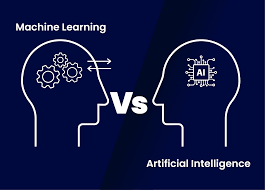
Even though Artificial Intelligence (AI) and Machine Learning (ML) are frequently mentioned together, they actually refer to different ideas. AI encompasses the wider area of developing systems that can imitate human intelligence, including abilities like reasoning, problem-solving, and learning. In contrast, ML is a part of AI that centers on training machines to learn from data and enhance their performance without direct programming. 

For instance, an AI program might utilize rule-based coding, like an expert system that adheres to predetermined steps for diagnosing an illness. On the other hand, a machine learning model would examine patient information, detect trends, and acquire the ability to make diagnoses independently.

Conclusion

Machine Learning is a key component in today’s technology, changing sectors and enhancing quality of life. Its uses range from self-driving cars and fraud detection systems to personalized online shopping experiences and advancements in healthcare, making its impacts widespread and significant. 

One of the most thrilling parts of machine learning is its constant development. Recent algorithms, tools, and frameworks are increasing accessibility, scalability, and power. Nevertheless, creating efficient ML models necessitates a solid grasp of the data, defined goals, and the capability to iterate and enhance. 

In the coming years, ML will keep influencing our technology use and problem-solving methods. Whether you are a developer, a business professional, or just interested, gaining knowledge of ML concepts, techniques, and applications leads to a world of opportunities. Now that you have this comprehensive guide and examples, you’re ready to discover the wonders of ML and its potential for transformation.